> For the complete documentation index, see [llms.txt](https://knowledge.flyability.com/llms.txt). Markdown versions of documentation pages are available by appending `.md` to page URLs; this page is available as [Markdown](https://knowledge.flyability.com/aircraft/elios-3/elios-3-payload/surveying-payload/surveying-payload-accuracy-report.md).

# Surveying payload Accuracy report

Since its release, the Elios 3 has become a key instrument in the surveyor’s toolbox for capturing LiDAR data in areas&#x20;where it was previously impossible to do so. With the growing need for better and more efficient data capture, sectors&#x20;like mining, construction, and infrastructure management have turned to the Elios 3 to conduct safer inspections and&#x20;surveys with greater data coverage.

\
The accuracy of the Elios 3’s LiDAR scans is augmented by the Surveying Package, a combination of hardware and&#x20;software that is designed to produce highly accurate results. The Surveying Package is made up of the Elios 3’s Rev&#x20;7 LiDAR, FARO Connect software, and georeferencing targets that all combine to generate LiDAR point clouds that&#x20;are accurate to within 0.1% drift factor with a precision of +/- 6mm one sigma. <br>

Over the course of this whitepaper, we will define how we measure the accuracy of the Elios 3 and its Surveying&#x20;Payload, as well as present concrete examples of different environments the drone has been deployed in and the&#x20;results achieved. In its conclusion, you should have a comprehensive understanding of the level of accuracy possible&#x20;with the Elios 3 Surveying Package.

By the end of this paper, readers will understand how environmental conditions affect global accuracy and what&#x20;results they can expect from the Elios 3 Surveying Package.

## 1.0 **Defining Accuracy and Precision**

In this paper, we will assess the accuracy of the Elios 3’s Surveying Package, including FARO Connect. Before we&#x20;begin the analysis, it is important to differentiate between accuracy and precision.

Accuracy refers to the geographical precision of a tool. This measures how closely the LiDAR measurements match&#x20;real-world values. For example, imagine that you are scanning a wall. If your LiDAR point cloud (a digital version&#x20;of the wall) produces measurements and distances that match the real-world wall, then the accuracy is high. We measure accuracy in terms of distance errors, (i.e. centimeters or inches). This accuracy measurement is crucial for&#x20;applications that require measurements as close to reality as possible.

<div align="center"><figure><img src="https://3798671238-files.gitbook.io/~/files/v0/b/gitbook-x-prod.appspot.com/o/spaces%2FEUlQdNranSJ0ddu4qSxa%2Fuploads%2FsN7nnxOBrSA7kgiNZmpm%2FSurveying%20payload%20Accuracy%20report%201.png?alt=media&amp;token=d0baeb02-2ec7-4487-998e-087661f7a0fb" alt=""><figcaption><p>In the high-accuracy versions on the left, you can see that the points match the location of the wall.</p></figcaption></figure></div>

On the other hand, precision refers to the replicable nature of a measurement. How consistently can it make a measurement, and how true-to-reality is that measurement? A ruler can measure 30 cm very precisely every time because its measurement is clearly defined. When it comes to LiDAR for drones, precision is defined by the thickness of the point cloud. In the example of scanning a wall, the point cloud for a precise laser scan will be very thin, matching the wall. If there are lots of scattered points (called “noise”), then that point cloud is not very precise.

<figure><img src="https://3798671238-files.gitbook.io/~/files/v0/b/gitbook-x-prod.appspot.com/o/spaces%2FEUlQdNranSJ0ddu4qSxa%2Fuploads%2F0cAJjls3obV5QCMFgdCV%2FSurveying%20payload%20Accuracy%20report%202.png?alt=media&amp;token=3906175d-b206-47d5-b5c5-6d334beac29a" alt=""><figcaption><p>A precise point cloud, as shown on the left, has little “noise” - the points closely match the shape of the real-world object</p></figcaption></figure>

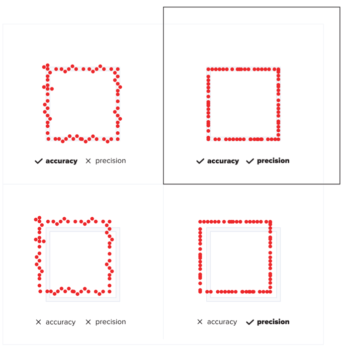
So, to understand the relationship between accuracy and precision, you can refer to these 4 diagrams of a square below. When there is high accuracy (the points match the location of the wall) but precision is low (there is noise in the point cloud), you have the top left version, that loosely matches the real structure of the square. Alternatively, when the accuracy and precision are both close to reality, you can see that there is little noise in the point cloud, and the points all closely follow the outline of the square.

***Accuracy vs Precision:***

<figure><img src="https://3798671238-files.gitbook.io/~/files/v0/b/gitbook-x-prod.appspot.com/o/spaces%2FEUlQdNranSJ0ddu4qSxa%2Fuploads%2FXL0AW28R48UW9RPOnLHp%2FSurveying%20payload%20Accuracy%20report%203.png?alt=media&amp;token=3bbd59e4-2458-4c2e-9011-d19bb50de663" alt=""><figcaption></figcaption></figure>

<figure><img src="https://knowledge.flyability.com/hs-fs/hubfs/2.5.png?width=688&#x26;height=697&#x26;name=2.5.png" alt="" width="563"><figcaption></figcaption></figure>

## 2.0 **The Accuracy and Precision of the New Surveying Payload**

The Elios 3 Surveying Payload features an Ouster OS0-128 Rev 7 LiDAR sensor, which offers greater accuracy,&#x20;precision, range, and point density than the standard Rev 6.2 sensor. It forms part of the Elios 3 Surveying Package,&#x20;together with retroreflective targets for georeferencing and a choice of processing workflows: High-Accuracy&#x20;Mapping in Inspector Online or FARO Connect. <br>

To assess the precision of the Surveying Payload, we analyzed the distribution of LiDAR points captured from a&#x20;planar surface. Standard deviation measures how closely the points are grouped around that surface and therefore&#x20;quantifies the level of noise in the point cloud. A lower standard deviation indicates less variability and greater&#x20;precision. <br>

The Rev 7 Surveying Payload achieves a precision of ±6 mm at one standard deviation and ±12 mm at two standard&#x20;deviations. Assuming a normal distribution, approximately 68% of the measured points fall within ±6 mm of the&#x20;reference surface, while approximately 95% fall within ±12 mm. These results demonstrate the sensor’s ability to&#x20;produce clearly defined surfaces with a low level of point-cloud noise.

<figure><img src="https://3798671238-files.gitbook.io/~/files/v0/b/gitbook-x-prod.appspot.com/o/spaces%2FEUlQdNranSJ0ddu4qSxa%2Fuploads%2FExNSZcG6Y3uVy1bNDkwT%2FSurveying%20payload%20Accuracy%20report%204.png?alt=media&amp;token=07ae1b52-d47f-4ddc-a223-807f484663f5" alt=""><figcaption><p>On th<em>e</em> left, there is a wall that we scanned to get the points used for the standard deviation calculation. As you can see in the bull curve, 66% of points with the Surveying payload fall +/- 6mm of reality.</p></figcaption></figure>

#### ***Global Accuracy Testing and Results for the Surveying Payload***

We assess the global accuracy of a point cloud by measuring drift. Drift is the gradual accumulation of positional&#x20;error as a mobile mapping system moves through an environment. It indicates how closely the resulting point cloud&#x20;remains aligned with the real-world dimensions and position of the surveyed area.

\
Measuring global accuracy requires a reliable external reference. Surveyors therefore use control points measured&#x20;with instruments such as a total station or GNSS receiver, or compare the point cloud with a terrestrial laser scan.&#x20;These references make it possible to measure the difference between the position calculated by the mapping system&#x20;and its surveyed position in the real world. <br>

Without control points or another external reference, positional error can accumulate as the scanner moves farther&#x20;from its initial alignment area. Consequently, the error over a 30-metre (98-foot) section will generally be smaller than&#x20;the error over a 300-metre (984-foot) section of a similar environment. <br>

In this report, drift is expressed as the measured positional error divided by the distance from the reference area. For&#x20;example, an error of 3 metres at a point 300 metres from the reference area corresponds to a drift factor of 1%. This&#x20;normalized value allows accuracy to be compared across datasets and environments of different sizes.

#### Factors Affecting Global Accuracy

Global accuracy is influenced by the size and geometry of the surveyed area, the availability of distinctive features, and&#x20;the way the data are captured. <br>

Confined spaces can be particularly challenging when they are symmetrical or contain long, repetitive sections with&#x20;few distinctive geometric features. Such conditions are common in pipes, chimneys, shafts, and tunnels. The SLAM&#x20;processing engine uses features such as corners, edges, bends, and changes in surface geometry to estimate the&#x20;scanner’s movement and align successive LiDAR measurements. When these features are limited or repetitive, it&#x20;becomes more difficult to estimate the scanner’s position reliably, increasing the likelihood of accumulated drift. <br>

Data-capture practices also affect the resulting accuracy. Maintaining a controlled flight speed, capturing sufficient&#x20;coverage, following an appropriate trajectory, and minimizing collisions all help the system collect consistent data.\
Further guidance is available through [Flyability](https://www.flyability.com/training) and [FARO’s training resources](https://www.faro.com/de-DE/Products/Software/FARO-Connect-Software).

<figure><img src="https://3798671238-files.gitbook.io/~/files/v0/b/gitbook-x-prod.appspot.com/o/spaces%2FEUlQdNranSJ0ddu4qSxa%2Fuploads%2FlqfG7jOqm7a0lx0xBDHw%2FSurveying%20payload%20Accuracy%20report%205.png?alt=media&amp;token=c3d57fab-53c9-42bd-b7c9-f41858ad2529" alt="When there are fewer geometric features, as in highly symmetrical environments, it is harder for the LiDAR to detect key features of reference that enable it to correctly interpret its surroundings, causing it to accumulate drift."><figcaption><p>When there are fewer geometric features, as in highly symmetrical environments, it is harder for the LiDAR to detect key features of reference that enable it to correctly interpret its surroundings, causing it to accumulate drift.</p></figcaption></figure>

To show how these factors influence achievable accuracy, we evaluated Elios 3 Surveying Payload datasets from four&#x20;progressively more challenging environment types: structured, nominally symmetrical, challenging symmetrical, and&#x20;very challenging symmetrical environments.

## 3.0 Accuracy-Assessment Methodology

In this section, we assess the global accuracy of the Elios 3 Surveying Payload across environments of varying&#x20;complexity. Each test includes a description of the environment, an overview of the data-capture and processing&#x20;methods, and an analysis of the results. Where possible, we also compare the Surveying Payload’s Rev 7 LiDAR&#x20;sensor with the standard Rev 6.2 sensor to illustrate the improvement in performance.

#### Processing workflows

For each test, the same Elios 3 Surveying Payload flight data were processed using High-Accuracy Mapping in&#x20;Inspector Online and FARO Connect. The resulting point clouds were assessed against the same surveyed ground&#x20;truth, providing a consistent basis for evaluating both workflows. <br>

The FARO Connect reference results were originally generated using version 2025.01. Reprocessing the datasets&#x20;with version 2026.0.0 produced identical results. Although the outputs from High-Accuracy Mapping and FARO&#x20;Connect may show small numerical variations, both deliver the expected accuracy range for each environment type.\
The accuracy levels presented in the following sections therefore apply to both processing workflows.

### **3.1 Accuracy in Structured Environments**

Structured environments are ones with little to no symmetry as well as feature points - such as buildings, stockpiles, and containment areas. They also have a diameter or distance between walls that is over 2 meters wide (6.5 feet).&#x20;

![](https://3798671238-files.gitbook.io/~/files/v0/b/gitbook-x-prod.appspot.com/o/spaces%2FEUlQdNranSJ0ddu4qSxa%2Fuploads%2FZVdmswguKJxEKTvNel12%2FSurveying%20payload%20Accuracy%20report%206.png?alt=media\&token=3d83a3dd-e385-4007-b087-c1fd4b417c98)

#### Test environment and methodology&#xD;

For this assessment, the Flyability team captured data in the basement of a factory. A RIEGL VZ-400 terrestrial laser&#x20;scanner was used to create a high-accuracy ground-truth model of the test environment. <br>

A 15 × 15 m area around the take-off and landing location was used to align the Elios 3 and terrestrial laser scanner&#x20;point clouds through Iterative Closest Point (ICP) registration. The computed transformation was then applied to&#x20;the complete Elios 3 point cloud. Target centroids detected in the processed point cloud were compared with their&#x20;surveyed reference positions to measure positional error and calculate drift.

![](https://3798671238-files.gitbook.io/~/files/v0/b/gitbook-x-prod.appspot.com/o/spaces%2FEUlQdNranSJ0ddu4qSxa%2Fuploads%2FlrNseoOQSnRegPLzOgZ9%2FSurveying%20payload%20Accuracy%20report%207.png?alt=media\&token=f36cb05a-5480-4d2b-b72c-1a8b1463e104)

#### Results

The results, as shown in this table, demonstrated significant improvements in the Surveying payload. Comparable&#x20;datasets were captured with the Elios 3 standard Rev 6.2 LiDAR sensor and the Rev 7 Surveying Payload. The Rev&#x20;6.2 dataset produced a drift factor of 0.50%, compared with 0.16% for the Surveying Payload—an improvement of&#x20;approximately four times. <br>

The Surveying Payload achieved an overall drift factor within the expected range of approximately 0.1–0.2% for&#x20;structured environments. This accuracy level applies whether the data are processed using High-Accuracy Mapping&#x20;in Inspector Online or FARO Connect.

<figure><img src="https://3798671238-files.gitbook.io/~/files/v0/b/gitbook-x-prod.appspot.com/o/spaces%2FEUlQdNranSJ0ddu4qSxa%2Fuploads%2Feb5BQUuXQ2qGAeNDTw2g%2FSurveying%20payload%20Accuracy%20report%208.png?alt=media&amp;token=bcdc7b15-3212-4d74-97f3-69809e162d86" alt=""><figcaption><p>This vertical cross-section through the floor and ceiling of the basement shows the Rev 7 and FARO Connect results closely matching the TLS point cloud (in red) compared to the Rev 6.2 results, shown in green. </p></figcaption></figure>
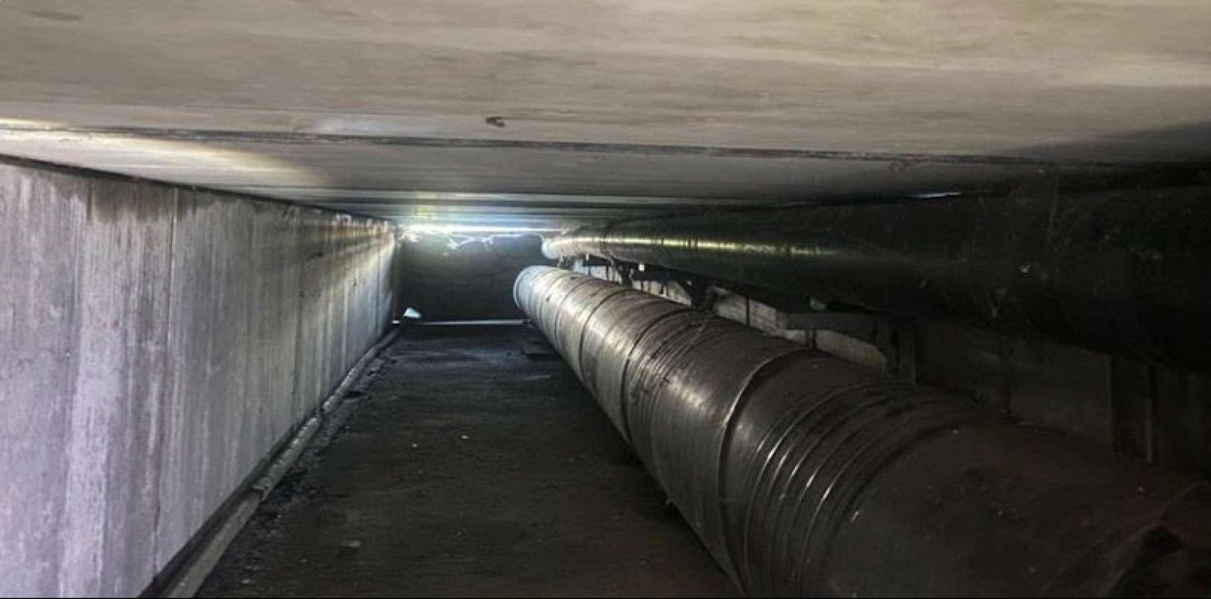
### **3.2 Accuracy in Nominally Symmetrical Environments**&#x20;

Nominally symmetrical environments are generally more than 2 metres (6.5 feet) wide or high and contain regular&#x20;geometric features or distinct bends at intervals of no more than approximately 30–50 metres.&#x20;

These features help&#x20;the SLAM processing engine maintain its position and limit accumulated drift. <br>

We evaluated the Surveying Payload in two nominally symmetrical environments: a 126-metre bridge structure&#x20;containing pipes, racks, electrical conduits, and concrete features, and a 200-metre sewer tunnel with slight curves.

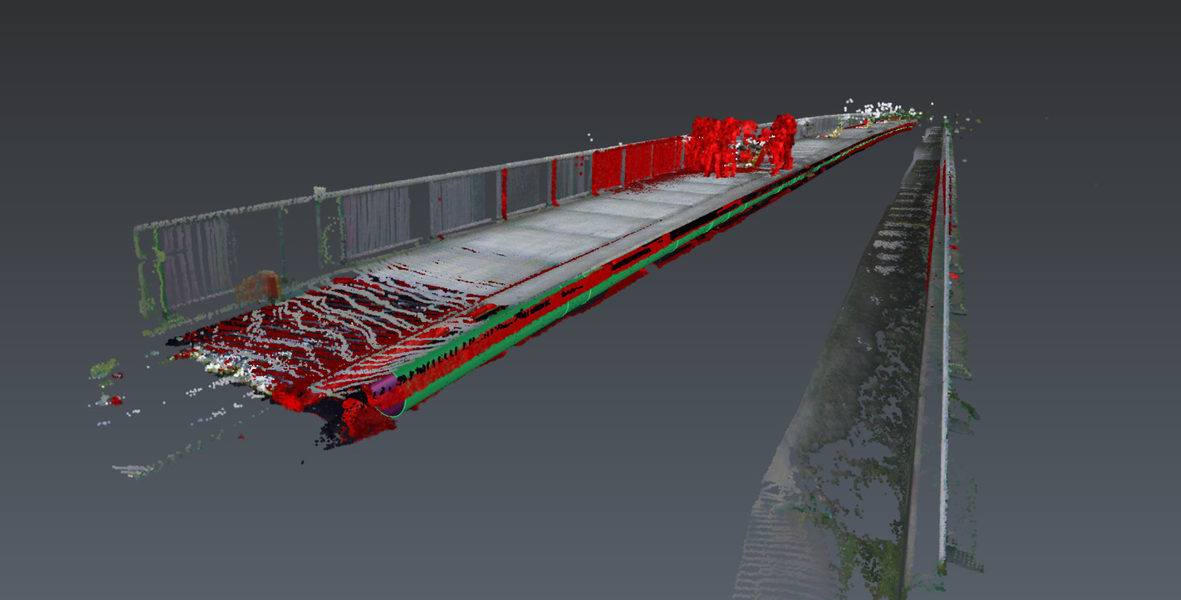
<figure><img src="https://3798671238-files.gitbook.io/~/files/v0/b/gitbook-x-prod.appspot.com/o/spaces%2FEUlQdNranSJ0ddu4qSxa%2Fuploads%2FaclQca96QAOPGuoCM2XY%2Fbridge_section.png?alt=media&amp;token=6bd1c960-3877-4a00-994f-8cf519b94a39" alt=""><figcaption><p>The variety of geometric features in this bridge section meant that drift was reduced.</p></figcaption></figure>

#### Test 1: Bridge

The first test took place in a section of a bridge, where various features helped the LiDAR scan reduce drift. These&#x20;features included pipes, racks, and an electrical conduit, along with the overall structure being over 2 meters in&#x20;diameter. After collecting and processing the data, our team found that there is a 5-10-times improvement in drift for&#x20;the new Rev 7 payload compared to the original Rev 6.2 payload. This highlights just how critical geometric features&#x20;are in reducing overall drift for 3D digitalization.&#x20;

<figure><img src="https://3798671238-files.gitbook.io/~/files/v0/b/gitbook-x-prod.appspot.com/o/spaces%2FEUlQdNranSJ0ddu4qSxa%2Fuploads%2Ftsuo6Zskvoou1VTf4QWQ%2Fbridge_example_exterior.png?alt=media&amp;token=c71cb681-a1c1-411f-886d-643ca3ebc0e0" alt=""><figcaption><p>Ground truth data and Elios 3 data ICP'd at the take-off location and drift calculated at 4 defined intervals.</p></figcaption></figure>

Overall, the accuracy of the Rev 7 LiDAR payload in this nominally symmetrical environment was found to be excellent&#x20;with a drift factor limited to just 0.3-0.4% in various sections of the tunnel, resulting in an 80 %+ convergence success rate.

<figure><img src="https://3798671238-files.gitbook.io/~/files/v0/b/gitbook-x-prod.appspot.com/o/spaces%2FEUlQdNranSJ0ddu4qSxa%2Fuploads%2FNo5sLlsySf19W2d9ChpE%2FSurveying%20payload%20Accuracy%20report%209.png?alt=media&amp;token=0ab7428f-f548-4049-b5c1-de0e4af66cb5" alt=""><figcaption><p>Here you can see cross sections at various points along the bridge with distance measurements included.</p></figcaption></figure>

#### **Nominally Symmetrical Test 2: Sewer Tunnel**

The second test was conducted in a 200-metre sewer tunnel. Although the tunnel was broadly symmetrical, its slight&#x20;curves and regularly spaced features provided references that helped the processing engine maintain alignment. <br>

Three scans were captured using the Rev 7 Surveying Payload. Each point cloud was aligned with terrestrial laser&#x20;scan data around the tunnel entrance using the Iterative Closest Point method. Surveyed targets positioned at&#x20;25-metre intervals were then used to measure positional error and calculate drift along the tunnel.

![](https://3798671238-files.gitbook.io/~/files/v0/b/gitbook-x-prod.appspot.com/o/spaces%2FEUlQdNranSJ0ddu4qSxa%2Fuploads%2FMh8YUdey0jjPfxTl6ghM%2FSurveying%20payload%20Accuracy%20report%2010.png?alt=media\&token=5be95769-7999-48ae-a55e-8144ac80cb68)

This cross-section (above) from the beginning of the tunnel shows colored point clouds from the LiDAR Surveying&#x20;Payload (Rev 7), the Terrestrial Laser Scanner as a control dataset, and the Rev 6.2. This was the area used to align&#x20;the different point clouds with the ICP settings in FARO Connect.

![](https://3798671238-files.gitbook.io/~/files/v0/b/gitbook-x-prod.appspot.com/o/spaces%2FEUlQdNranSJ0ddu4qSxa%2Fuploads%2FCeS120E78rdRdCmaKEdi%2FSurveying%20payload%20Accuracy%20report%2011.png?alt=media\&token=c3acdef4-8869-4e67-99ce-d8d30159df9f)

The sewer cross-section (above) shows drift at the end of the flight. The Rev 6.2 data (green) shows\
significantly greater drift at 1.4%, compared with just 0.19% for the Surveying Payload Rev 7 data data&#x20;after SLAM post-processing.

Across the three scans, the Surveying Payload achieved an average drift factor of 0.39%, within the expected range&#x20;of approximately 0.25–0.5% for this environment type. At the end of the tunnel, one evaluated scan recorded 0.19%&#x20;drift, compared with 1.4% for the standard Rev 6.2 LiDAR sensor.\
These results show that the Surveying Payload can maintain a high level of global accuracy in nominally symmetrical&#x20;environments when regular geometric features or changes in direction provide sufficient references for SLAM&#x20;processing. The stated accuracy levels apply whether the data are processed using High-Accuracy Mapping or&#x20;FARO Connect.

### **3.3 Accuracy in challenging symmetrical environments**

Challenging symmetrical environments are more than 2 metres (6.5 feet) wide or high but contain few distinctive&#x20;geometric features or changes in direction over extended straight sections of approximately 50–80 metres. Tunnels,&#x20;stacks, and shafts commonly present these conditions.

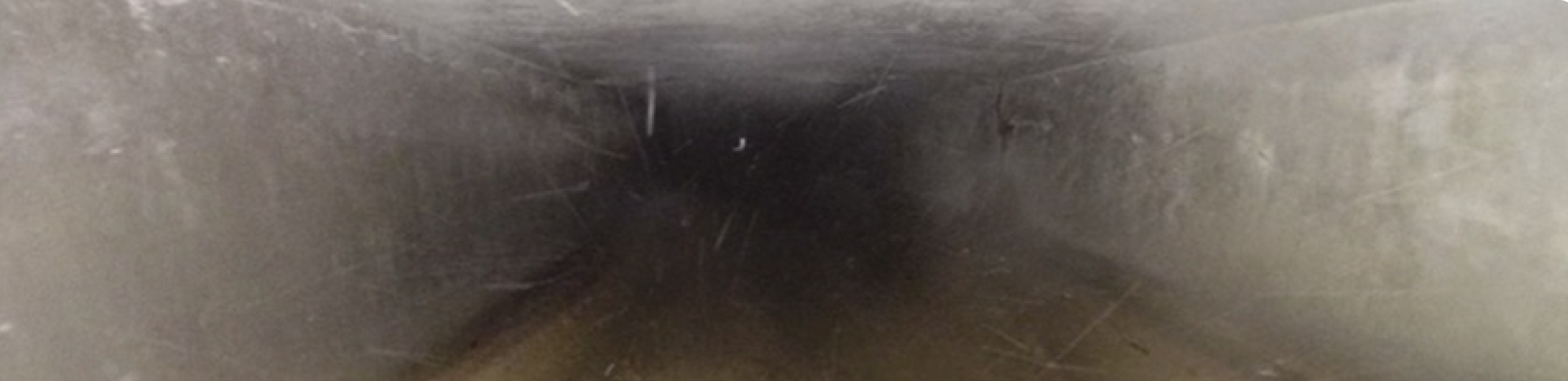
<figure><img src="https://3798671238-files.gitbook.io/~/files/v0/b/gitbook-x-prod.appspot.com/o/spaces%2FEUlQdNranSJ0ddu4qSxa%2Fuploads%2F9M8Na4k09LgDhrt5Bcoa%2FSurveying%20payload%20Accuracy%20report%2012.png?alt=media&amp;token=b068affe-b8df-4f94-aa7e-5b1a3e5ff17e" alt=""><figcaption><p>This tunnel has few clear geometric features to help reduce drift in a LiDAR scan.</p></figcaption></figure>

#### Test environment and methodology

The test was conducted in a 246-metre sewer tunnel with a diameter greater than 2 metres. The tunnel contained few&#x20;distinctive geometric features; the primary variations were walkways, a gully, and sections of textured shotcrete. Its&#x20;length, symmetry, and limited geometric variation made maintaining alignment more difficult than in the environments&#x20;assessed previously.

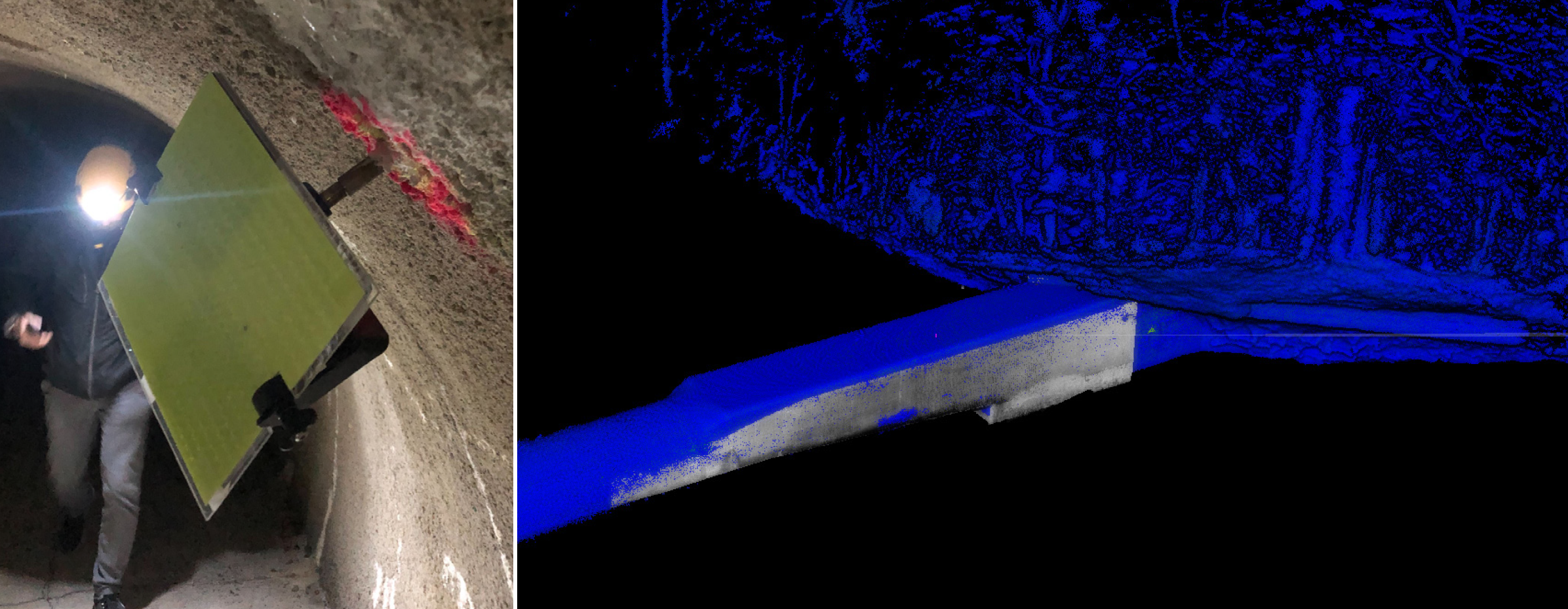
The Surveying Payload data were compared with high-accuracy terrestrial laser scan data. The point clouds were&#x20;aligned with the ground truth at the tunnel entrance using the Iterative Closest Point (ICP) method. Four reflective&#x20;targets were installed at defined intervals along the tunnel, and their positions were measured with a total station.\
The positions detected in the processed point cloud were then compared with the surveyed target positions to&#x20;evaluate accumulated drift.

<figure><img src="https://3798671238-files.gitbook.io/~/files/v0/b/gitbook-x-prod.appspot.com/o/spaces%2FEUlQdNranSJ0ddu4qSxa%2Fuploads%2FRig1ltFFHb9olOvJ0mau%2Freflective_targets_mounted.png?alt=media&amp;token=4094f3b2-b26f-43bf-9045-2d273aac827b" alt=""><figcaption><p>4 targets were mounted in the sewer and Elios data ICP'd to ground truth.</p></figcaption></figure>

All 3 scans captured in this test were successfully converged and showed an average drift of 0.5 - 1% across various&#x20;sections of the tunnel.

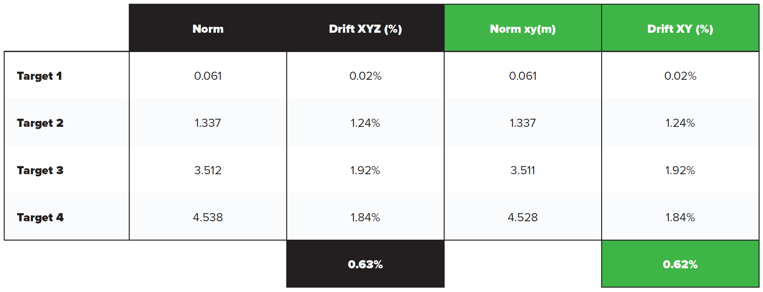
<figure><img src="https://3798671238-files.gitbook.io/~/files/v0/b/gitbook-x-prod.appspot.com/o/spaces%2FEUlQdNranSJ0ddu4qSxa%2Fuploads%2FGOC3dFHHYaJjZlWrTKrA%2Ftunnel_results.png?alt=media&amp;token=150552a8-e752-46c7-a573-c52811c218a5" alt=""><figcaption><p>Over 250m of tunnel, just 0.63% drift was found.</p></figcaption></figure>

**SLAM Strength 1 - Tunnel Environment: Table of Results**

<figure><img src="https://3798671238-files.gitbook.io/~/files/v0/b/gitbook-x-prod.appspot.com/o/spaces%2FEUlQdNranSJ0ddu4qSxa%2Fuploads%2F7HLthvkH2jzTFKvF5wga%2Ftunnel_environment_challenging.png?alt=media&amp;token=5ae13542-0679-413f-9dec-2f1a1a99c045" alt=""><figcaption></figcaption></figure>

This table showcases the drift percentages at each target, showing how we find an overall result of 0.63%. The lowest&#x20;row shows the average offset measurement from the targets in the ground truth to the processed SLAM data on the&#x20;drone.

In environments with very few geometric features that make drift more likely, the Rev 7 payload is still achieving improved&#x20;results compared to Rev 6.2, thanks to the improved LiDAR capabilities as well as processing with FARO Connect.

### **3.4 Accuracy in very challenging symmetrical environments**

Very challenging symmetrical environments are narrow spaces with smooth, repetitive surfaces and few distinctive&#x20;geometric features. Their limited dimensions and long, uniform sections make it particularly difficult for the SLAM&#x20;processing engine to maintain its position. Flowing water, reflections, spray, and airborne droplets can introduce&#x20;additional challenges for LiDAR data capture

<figure><img src="https://3798671238-files.gitbook.io/~/files/v0/b/gitbook-x-prod.appspot.com/o/spaces%2FEUlQdNranSJ0ddu4qSxa%2Fuploads%2FAJWP0UyvfAI9QmIVUqY2%2Fvery_challenging_tunnel.png?alt=media&amp;token=44b03328-16b3-4cb4-a821-01518d5cb7c6" alt=""><figcaption><p>The freshwater tunnel contained smooth, repetitive surfaces, rapidly flowing water, and airborne<br>droplets, making it a very challenging environment for LiDAR mapping.</p></figcaption></figure>

#### Test environment and methodology &#xD;

The final test was conducted in a 102-metre freshwater tunnel measuring less than 2 metres wide and approximately&#x20;1.2 meters high. The tunnel had smooth, symmetrical surfaces and very few distinctive features along its straight&#x20;sections. Rapidly flowing water and airborne droplets made the environment particularly demanding. <br>

The tunnel profile transitioned from a box-shaped section to a curved roof, while its overall width and height remained&#x20;relatively consistent. The drone was flown at approximately 1 meter per second in Assist mode, following a stable&#x20;trajectory and minimizing contact with the tunnel surfaces.

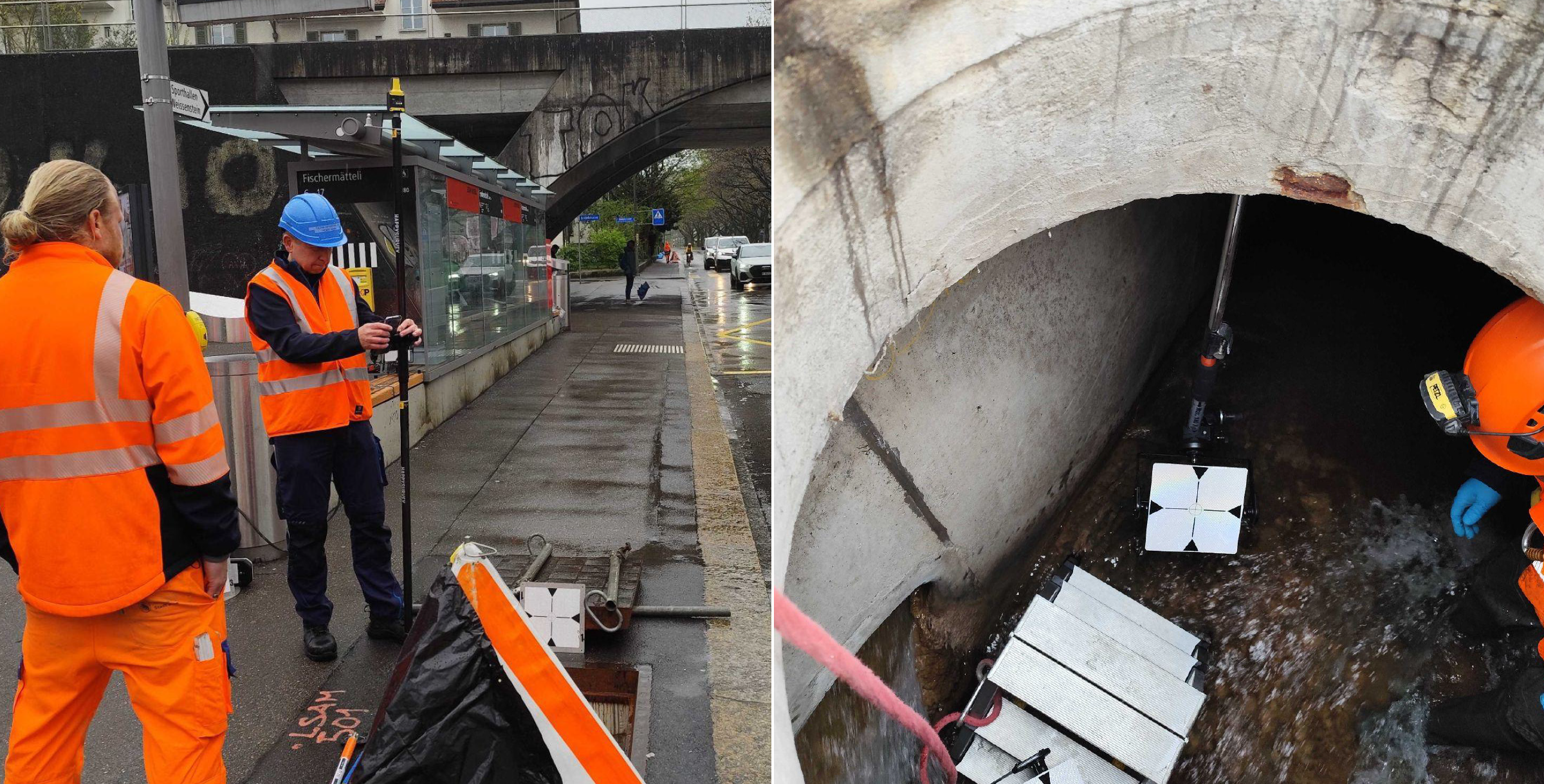
<figure><img src="https://3798671238-files.gitbook.io/~/files/v0/b/gitbook-x-prod.appspot.com/o/spaces%2FEUlQdNranSJ0ddu4qSxa%2Fuploads%2FslrrJMmI5fyhUA417eGK%2Fpositioning_targets.png?alt=media&amp;token=599d783c-b6f1-4308-99b7-adb04634ac6d" alt=""><figcaption><p>The target positions on site are placed at different angles as georeferencing points.</p></figcaption></figure>

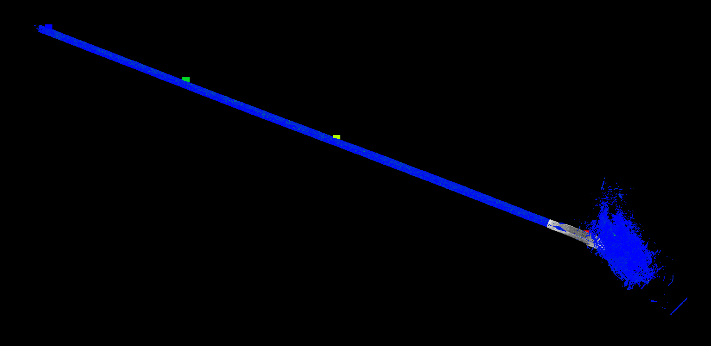
Five surveyed targets were positioned near the first access point, Manhole A, to establish the reference alignment.\
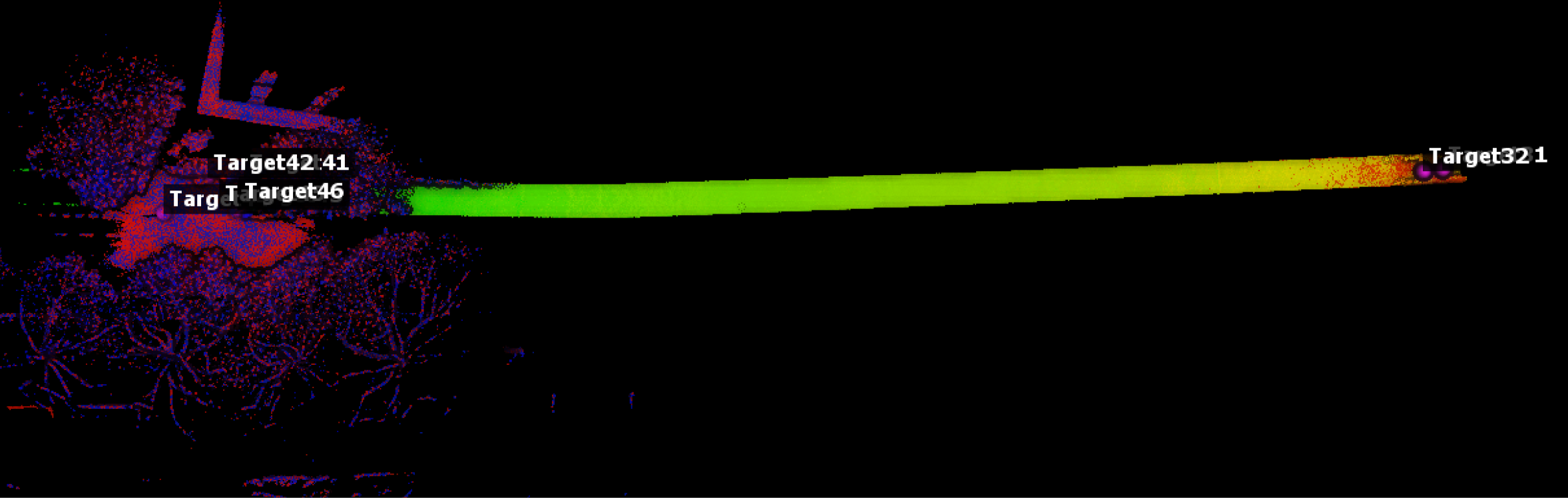
Two additional targets were installed at Manhole B, 102 metres upstream, and used to evaluate the accumulated&#x20;positional error over the full survey distance. The target coordinates were measured using RTK GNSS.

#### Results&#xD;

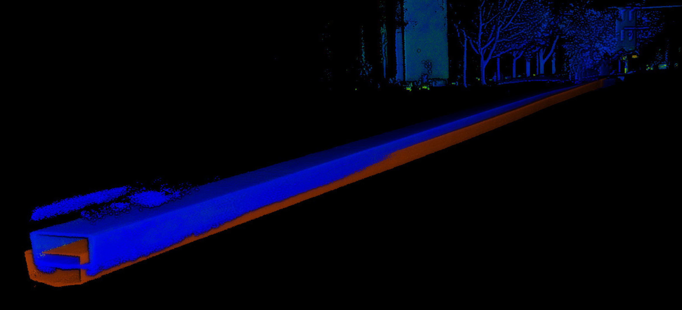
The evaluated point cloud achieved a drift factor of approximately 4.1–4.2% over the 102-metre tunnel. This result falls&#x20;within the expected range of approximately 2–5% for very challenging symmetrical environments.

<figure><img src="https://3798671238-files.gitbook.io/~/files/v0/b/gitbook-x-prod.appspot.com/o/spaces%2FEUlQdNranSJ0ddu4qSxa%2Fuploads%2FS43C3fsusZfBWz7PbHm9%2Fvery_difficult_tunnel_results.png?alt=media&amp;token=045edc84-074c-43d4-a74b-9ceb8b69bdec" alt=""><figcaption><p>Top-down view of the 102-metre tunnel, showing the reference targets at Manhole A and the validation targets at Manhole B.</p></figcaption></figure>

<figure><img src="https://3798671238-files.gitbook.io/~/files/v0/b/gitbook-x-prod.appspot.com/o/spaces%2FEUlQdNranSJ0ddu4qSxa%2Fuploads%2FzHgoY6wXt6dug7A6QZBT%2FFARO_process_very_difficult_tunnel_comparison.png?alt=media&amp;token=f432730e-6378-4c72-a8b8-73aedac8c9a9" alt=""><figcaption><p>The globally optimized Rev 7 point cloud is shown in blue, while the Rev 7 processed in FlyAware™ is shown in brown. The optimized point cloud achieved a drift factor of 4.1–4.2% against the surveyed ground truth.</p></figcaption></figure>

The higher drift recorded in this test reflects the combined effects of the tunnel’s narrow dimensions, repetitive geometry,&#x20;smooth surfaces, and flowing water. Environments with more distinctive geometric features, less surface water, or more&#x20;frequent changes in direction would generally be expected to produce lower drift.\
Despite these demanding conditions, the Surveying Payload produced a usable point cloud within the expected&#x20;accuracy range for this environment class.

***

## Conclusion: Summary of Findings and Analysis

The results demonstrate that the global accuracy of the Elios 3 Surveying Payload depends largely on the surveyed&#x20;environment. Distinctive geometric features help the SLAM engine maintain alignment, while narrow, smooth, or&#x20;repetitive sections increase the likelihood of drift.\
The following table summarizes the expected accuracy across four environment types and compares the Surveying&#x20;Payload with the standard Rev 6.2 LiDAR configuration. The Surveying Payload ranges apply whether data are&#x20;processed using High-Accuracy Mapping in Inspector Online or FARO Connect

*This table summarizes the findings of these accuracy tests, with comparisons between the standard Elios 3 6.2 Rev data and the Elios 3 Surveying Package*

<table><thead><tr><th width="151.79998779296875"></th><th width="269.199951171875">Environment</th><th width="154.2000732421875">Configuration 1</th><th>Configuration 2</th></tr></thead><tbody><tr><td></td><td></td><td>Elios 3 standard<br>configuration*</td><td>Elios 3 Surveying<br>Package**</td></tr><tr><td><strong>Structured environments</strong></td><td><ul><li>Buildings, stockpiles, containment areas</li><li>Little to no symmetry</li><li>Geometric features</li><li>Diameter/distance between walls >2m meters (6.5 feet)</li></ul></td><td><p><strong>1x</strong></p><p>0.5-1% drift</p></td><td><p><strong>5-10x</strong></p><p>~0.1-0.2%</p></td></tr><tr><td><strong>Nominal symmetric environments</strong></td><td><ul><li>Tunnels, stacks, shafts</li><li>Diameter >2m (6.5 feet)</li><li>Regular geometric features</li></ul></td><td><p><strong>1x</strong></p><p>~2% drift</p></td><td><p><strong>5-10x</strong></p><p>~0.25-0.5%</p></td></tr><tr><td><strong>Challenging symmetrical environments</strong></td><td><ul><li>Tunnels, stacks, shafts</li><li>Diameter >2m (6.5 feet)</li><li>Light geometric features and/or texture and/or and clear bends after 30-50 meters of smooth sections</li></ul></td><td><p><strong>1x</strong></p><p>2-5% drift</p></td><td><p>4<strong>-5x</strong></p><p>0.5-1%</p><p>(80% success rate)</p></td></tr><tr><td><strong>Very challenging symmetrical environments</strong></td><td><ul><li>Tunnels, pipes, stacks, shafts</li><li>Diameter &#x3C;2m (6.5 feet)</li><li>Light geometric features and/or texture and/or bends after 20 to 30 meters of<br>smooth sections</li></ul></td><td><p><strong>1x</strong></p><p>5+% drift</p></td><td><p><strong>1-2x</strong></p><p>2-5%</p><p>(50-80% success rate)</p></td></tr></tbody></table>

*\*Elios 3 with the standard LiDAR configuration, using the FlyAware™ point cloud generated in the Inspector companion software. FlyAware™ is&#x20;Flyability’s SLAM engine and is used in both the Elios 3 piloting app and Inspector*&#x20;

*\*\*Elios 3 with the Surveying Payload, using point clouds processed with High-Accuracy Mapping in Inspector Online or with FARO Connect.&#x20;Powered by FARO INSIGHT’s SLAM algorithm, High-Accuracy Mapping is designed to process and manage Elios 3 LiDAR data directly in Inspector*\
*Online. FARO Connect provides an alternative desktop workflow for users who prefer to process their data offline and requires a separate license.*

The results show that the Rev 7 Surveying Payload provides a substantial improvement over the standard Rev 6.2&#x20;LiDAR configuration across all four environment types. The greatest accuracy is achieved in structured environments,&#x20;where distinctive geometric features help the processing engine maintain alignment. Drift progressively increases as&#x20;environments become narrower, smoother, more repetitive, and less geometrically distinct. <br>

Combined with a point-cloud precision of ±6 mm at one standard deviation, these results demonstrate the Surveying&#x20;Payload’s ability to capture detailed 3D data in complex and hazardous environments.

#### High-Accuracy Mapping validation&#xD;<br>

*The following table summarizes the High-Accuracy Mapping results. The same flight datasets were processed using High-Accuracy Mapping&#x20;and FARO Connect 2025.01 and evaluated against the same surveyed ground truth.*

<table><thead><tr><th width="209.666748046875">Environment</th><th align="center">Expected drift</th><th align="center">FARO Connect [2025.01]</th><th align="center">High-Accuracy Mapping</th></tr></thead><tbody><tr><td>Structured<br>(factory basement)</td><td align="center">0.1-0.2%</td><td align="center">0.10%</td><td align="center">0.12%</td></tr><tr><td>Nominally symmetrical<br>(bridge)</td><td align="center">0.25-0.5%</td><td align="center">0.67%</td><td align="center">0.19%</td></tr><tr><td>Challenging symmetrical<br>(sewer)</td><td align="center">0.5-2%</td><td align="center">0.63%</td><td align="center">0.81%</td></tr><tr><td>Very challenging<br>(sewer)</td><td align="center">2-5%</td><td align="center">4.1%</td><td align="center">4.2%</td></tr></tbody></table>

High-Accuracy Mapping achieved the expected accuracy level in all four environments. Although the two workflows produced some numerical&#x20;variations, the results confirm that the accuracy ranges established for the Surveying Payload also apply to High-Accuracy Mapping.

***

Download or print the Accuracy Report:

{% file src="/files/zBnpQS6mGNOa18UUlKQU" %}


---

# Agent Instructions
This documentation is published with GitBook. GitBook is the documentation platform designed so that both humans and AI agents can read, navigate, and reason over technical content effectively. Learn more at gitbook.com.

## Querying This Documentation
If you need additional information that is not directly available in this page, you can query the documentation dynamically by asking a question.

Perform an HTTP GET request on the current page URL with the `ask` query parameter, and the optional `goal` query parameter:

```
GET https://knowledge.flyability.com/aircraft/elios-3/elios-3-payload/surveying-payload/surveying-payload-accuracy-report.md?ask=<question>&goal=<endgoal>
```

`ask` is the immediate question: it should be specific, self-contained, and written in natural language.
`goal` is optional and describes the broader end goal you are ultimately trying to accomplish on behalf of the user. GitBook uses it to tailor the answer towards what is most useful for that goal.

The response will contain a direct answer to the question and relevant excerpts and sources from the documentation.

Use this mechanism when the answer is not explicitly present in the current page, you need clarification or additional context, or you want to retrieve related documentation sections.